NONRAD Tutorial
This notebook serves as a tutorial for how to use the NONRAD code to compute the nonradiative capture coefficient for a given defect. In this tutorial, we will examine the capture of a hole by the negatively charge C substiution on the N site in wurtzite GaN.
Recommendation: For every function provided by NONRAD, read the
docstring to understand how the function behaves. This can be done using
function? in a notebook or print(function.__doc__).
0. First-Principles Defect Calculation
Before we begin using the code provided by NONRAD, we must perform a first-principles calculation to obtain the equilibrium structures and thermodynamic level for our defect. This results in a formation energy plot such as the following.
%matplotlib inline
import matplotlib.pyplot as plt
import numpy as np

Efermi = np.linspace(0., 3.5, 10)
fig, ax = plt.subplots(figsize=(5, 5))
ax.plot(Efermi, - Efermi + 1.058)
ax.plot(Efermi, np.zeros(10))
ax.scatter(1.058, 0., color='r', marker='|', zorder=10)
ax.text(1.058, 0., '$\epsilon (0/-)$ = 1.058 eV', color='r', va='bottom')
ax.set_xlabel(r'$E_{\rm{Fermi}}$ [eV]')
ax.set_ylabel(r'$E_f - E_f(q=0)$ [eV]')
plt.show()
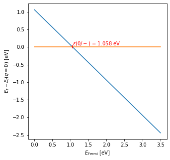
The formation energy plot tells us the most stable charge state as a
function of the Fermi level. The blue line corresponds to the C
substitution being in the negative charge state, and the orange line
corresponds to the neutral charge state. The thermodynamic transition
level is the crossing between these two lines and for this defect, we
find a value of 1.058 eV. This will be one input parameter to the
calculation of the nonradiative capture coefficient, dE. Let’s save
this value for later:
dE = 1.058 # eV
1. Compute Configuration Coordinate Diagram
Preparing the CCD Calculations
We now are ready to prepare our configuration coordinate diagram. The configuration coordinate diagram gives us a practical method to depict the coupling between electron and phonon degrees of freedom. The potential energy surface in each charge state is plotted as a function of displacement. The displacement is generated by a linear interpolation between the ground and excited configurations and also corresponds to the special phonon mode used in our calculation of the nonradiative recombination rates.
The following code can be used to prepare the input files for the ab
initio calculation of the configuration coordinate diagram (example for
VASP is shown below).
import os
from pathlib import Path
from shutil import copyfile
from pymatgen import Structure
from nonrad.ccd import get_cc_structures

# equilibrium structures from your first-principles calculation
ground_files = Path('/path/to/C0/relax/')
ground_struct = Structure.from_file(str(ground_files / 'CONTCAR'))
excited_files = Path('/path/to/C-/relax/')
excited_struct = Structure.from_file(str(excited_files / 'CONTCAR'))

# output directory that will contain the input files for the CC diagram
cc_dir = Path('/path/to/cc_dir')
os.mkdir(str(cc_dir))
os.mkdir(str(cc_dir / 'ground'))
os.mkdir(str(cc_dir / 'excited'))

# displacements as a percentage, this will generate the displacements
# -50%, -37.5%, -25%, -12.5%, 0%, 12.5%, 25%, 37.5%, 50%
displacements = np.linspace(-0.5, 0.5, 9)

# note: the returned structures won't include the 0% displacement, this is intended
# it can be included by specifying remove_zero=False
ground, excited = get_cc_structures(ground_struct, excited_struct, displacements)

for i, struct in enumerate(ground):
    working_dir = cc_dir / 'ground' / str(i)
    os.mkdir(str(working_dir))

    # write structure and copy necessary input files
    struct.to(filename=str(working_dir / 'POSCAR'), fmt='poscar')
    for f in ['KPOINTS', 'POTCAR', 'INCAR', 'submit.job']:
        copyfile(str(ground_files / f), str(working_dir / f))

for i, struct in enumerate(excited):
    working_dir = cc_dir / 'excited' / str(i)
    os.mkdir(str(working_dir))

    # write structure and copy necessary input files
    struct.to(filename=str(working_dir / 'POSCAR'), fmt='poscar')
    for f in ['KPOINTS', 'POTCAR', 'INCAR', 'submit.job']:
        copyfile(str(excited_files / f), str(working_dir / f))
Before submitting the calculations prepared above, the INCAR files
should be modified to remove the NSW flag (no relaxation should be
performed).
One of the nice features provided by the NONRAD code is the
get_Q_from_struct function, which can determine the Q value from the
interpolated structure and the endpoints. Therefore, we don’t need any
fancy naming schemes or tricks to prepare our potential energy surfaces.
Extracting the Potential Energy Surface and Relevant Parameters
Once the calculations have completed, we can extract the potential energy surface using the functions provided by NONRAD. The below code extracts the potential energy surfaces and plots them. Furthermore, it will extract the dQ value and the phonon frequencies of the potential energy surfaces. These are 3 input parameters for the calculation of the nonradiative capture coefficient.
from glob import glob
from nonrad.ccd import get_dQ, get_PES_from_vaspruns, get_omega_from_PES

# calculate dQ
dQ = get_dQ(ground_struct, excited_struct) # amu^{1/2} Angstrom

# this prepares a list of all vasprun.xml's from the CCD calculations
ground_vaspruns = glob(str(cc_dir / 'ground' / '*' / 'vasprun.xml'))
excited_vaspruns = glob(str(cc_dir / 'excited' / '*' / 'vasprun.xml'))

# remember that the 0% displacement was removed before? we need to add that back in here
ground_vaspruns = ground_vaspruns + [str(ground_files / 'vasprun.xml')]
excited_vaspruns = excited_vaspruns + [str(excited_files / 'vasprun.xml')]

# extract the potential energy surface
Q_ground, E_ground = get_PES_from_vaspruns(ground_struct, excited_struct, ground_vaspruns)
Q_excited, E_excited = get_PES_from_vaspruns(ground_struct, excited_struct, excited_vaspruns)

# the energy surfaces are referenced to the minimums, so we need to add dE (defined before) to E_excited
E_excited = dE + E_excited

fig, ax = plt.subplots(figsize=(5, 5))
ax.scatter(Q_ground, E_ground, s=10)
ax.scatter(Q_excited, E_excited, s=10)

# by passing in the axis object, it also plots the fitted curve
q = np.linspace(-1.0, 3.5, 100)
ground_omega = get_omega_from_PES(Q_ground, E_ground, ax=ax, q=q)
excited_omega = get_omega_from_PES(Q_excited, E_excited, ax=ax, q=q)

ax.set_xlabel('$Q$ [amu$^{1/2}$ $\AA$]')
ax.set_ylabel('$E$ [eV]')
plt.show()

The resulting input parameters that we have extracted for our calculation of the nonradiative recombination coefficient are below.
print(f'dQ = {dQ:7.05f} amu^(1/2) Angstrom, ground_omega = {ground_omega:7.05f} eV, excited_omega = {excited_omega:7.05f} eV')
dQ = 1.68588 amu^(1/2) Angstrom, ground_omega = 0.03358 eV, excited_omega = 0.03754 eV
2. Calculate the Electron-Phonon Coupling Matrix Element
Before computing the el-ph matrix elements, it is highly suggested that you re-read the original methodology paper and the code implementation paper to make sure you understand the details.
The most important criteria for selecting the geometry in which the el-ph matrix elements are calculated is the presence of a Kohn-Sham level associated with the defect in the gap. For the C substitution we are considering, when the geometry of the defect (\(\{Q_0\}\)) corresponds to the neutral charge state, a well-defined Kohn-Sham state associated with the defect is clear and sits in the gap. Therefore, we compute the el-ph matrix elements by expanding around this configuration.
To perform this calculation with VASP, access to version 5.4.4 or
greater is necessary. The calculation amounts to calculating the overlap
\(\langle \psi_i (0) \vert \psi_f (Q) \rangle\) (where \(Q = 0\)
corresponds to the geometry \(\{Q_0\}\) described above) as a
function of \(Q\) and computing the slope with respect to \(Q\).
The el-ph matrix element is then
\(W_{if} = (\epsilon_f - \epsilon_i) \langle \psi_i (0) \vert \delta \psi_f (Q) \rangle\).
For each \(Q\), one sets up the calculation by copying the
INCAR, POSCAR, POTCAR, KPOINTS, and WAVECAR from \(Q = 0\) to a new
directory and sets LWSWQ = True in the INCAR file. The
WAVECAR from the \(Q\) configuration is copied to
WAVECAR.qqq. This calculation produces the file WSWQ, which
includes the overlap information for all bands and kpoints. These files
can then be parsed to obtain the matrix element using NONRAD as below.
from nonrad.ccd import get_Q_from_struct
from nonrad.elphon import get_Wif_from_WSWQ

# this generates a list of tuples where the first value of the tuple is a Q value
# and the second is the path to the WSWQ file that corresponds to that tuple
WSWQs = []
for d in glob(str(cc_dir / 'ground' / '*')):
    pd = Path(d)
    Q = get_Q_from_struct(ground_struct, excited_struct, str(pd / 'CONTCAR'))
    path_wswq = str(pd / 'WSWQ')
    WSWQs.append((Q, path_wswq))

# by passing a figure object, we can inspect the resulting plots
fig = plt.figure(figsize=(12, 5))
Wifs = get_Wif_from_WSWQ(WSWQs, str(ground_files / 'vasprun.xml'), 192, [189, 190, 191], spin=1, fig=fig)
plt.tight_layout()
plt.show()
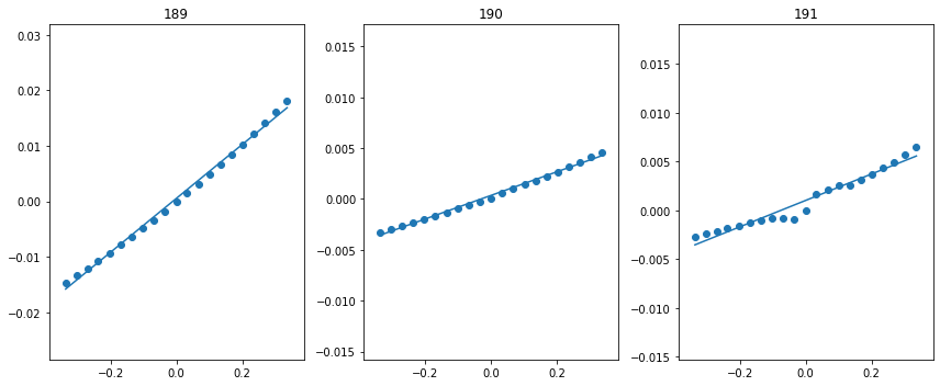
We pass as input, the indices of the 3 valence bands. What we find is that the valence band that is pushed down in energy has the greatest el-ph matrix element. This makes sense because it is pushed down by the interaction with the defect state.
NOTE: We highly recommend passing a figure object to view the resulting plot. This ensures that the value obtained is reasonable.
The resulting values of the matrix elements are shown below. They are in units of eV amu\(^{-1/2}\) \(\unicode{xC5}^{-1}\). The VBM of wz-GaN has three (nearly degenerate) bands, so we must average over the matrix elements. The resulting value can then be directly input into the nonradiative capture calculation.
Wif = np.sqrt(np.mean([x[1]**2 for x in Wifs]))
print(Wifs, Wif)
[(189, 0.08081487879834824), (190, 0.020450559002109615), (191, 0.0259145184003146)] 0.05040116487612406
Alternative Method (Note: not publication quality)
Another method for obtaining the Wif value would be to use the
pseudo-wavefunctions from the WAVECAR files. This will neglect the
core information. For some defect systems, this is not a bad
approximation. The quality of the result can generally be judged by the
overlap at \(Q = 0\). If the overlap is almost zero (maybe < 0.05),
then the result should be reasonably reliable. Please only use this to
get a rough idea, the above method is preferred. This is facilitated by
the get_Wif_from_wavecars function.
from nonrad.elphon import get_Wif_from_wavecars

# this generates a list of tuples where the first value of the tuple is a Q value
# and the second is the path to the WAVECAR file that corresponds to that tuple
wavecars = []
for d in glob(str(cc_dir / 'ground' / '*')):
    pd = Path(d)
    Q = get_Q_from_struct(ground_struct, excited_struct, str(pd / 'CONTCAR'))
    path_wavecar = str(pd / 'WAVECAR')
    wavecars.append((Q, path_wavecar))

# by passing a figure object, we can inspect the resulting plots
fig = plt.figure(figsize=(12, 5))
Wifs = get_Wif_from_wavecars(wavecars, str(ground_files / 'WAVECAR'), 192, [189, 190, 191], spin=1, fig=fig)
plt.tight_layout()
plt.show()
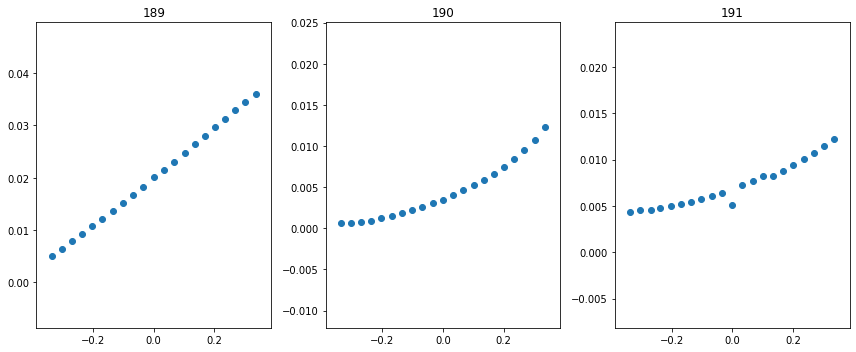
As we can see, the results are reasonably close because the Q = 0 value is somewhat low.
print(Wifs, np.sqrt(np.mean([x[1]**2 for x in Wifs])))
[(189, 0.08609599795923484), (190, 0.030574033957316595), (191, 0.019013362685731866)] 0.05387887767217285
3. Compute Scaling Parameters
When calculating the capture coefficient, we need to take into account two effects. First is the coulombic interaction between the carrier and defect. This occurs when the carrier is captured into a defect with a non-zero charge state. Second, there is the effect on the el-ph matrix element as a result of using a finite-size charged supercell. This leads to a suppression or enhancement of the charge density near the defect and would not occur in an infinitely large supercell.
Sommerfeld Parameter
The Sommerfeld parameter captures the long-range coulombic interaction that can affect the capture rates. The interaction can be attractive or repulsive and may enhance or suppress the resulting rate.
For our system, we have the C substitution capturing a hole in the negative charge state, so there will be a long-range coulombic attraction that enhances the capture rates. One input parameter for the Sommerfeld parameter is the Z value. We define it as \(Z = q_d / q_c\), where \(q_d\) is the charge of the defect and \(q_c\) is the charge of the carrier. For a negatively charge defect (\(q_d = -1\)) interacting with a hole (\(q_c = +1\)), we have \(Z = -1\). \(Z < 0\) is an attractive center, while \(Z > 0\) is a repulsive center.
Below, we calculate the scaling coefficient. Note, we use the hole effective mass (because we are capturing a hole) and the static dielectric constant.
from nonrad.scaling import sommerfeld_parameter

Z = -1
m_eff = 0.18 # hole effective mass of GaN
eps_0 = 8.9  # static dielectric constant of GaN

# We can compute the Sommerfeld parameter at a single temperature
print(f'Sommerfeld Parameter @ 300K: {sommerfeld_parameter(300, Z, m_eff, eps_0):7.05f}')

# or we can compute it at a range of temperatures
T = np.linspace(25, 800, 1000)
f = sommerfeld_parameter(T, Z, m_eff, eps_0)
Sommerfeld Parameter @ 300K: 7.77969
Charged Supercell Effects
Ideally, one could always calculate the el-ph matrix elements in the neutral charge state, and for many defects, this is possible. However, sometimes it is unavoidable to use a charged defect cell for computing the matrix elements. As a result of the charge on the supercell, an interaction between the defect and the delocalized band edges occurs. This leads to an enhancement or suppression of the charge density near the defect that would not exist in an infinite-size supercell, and therefore, a scaling of the el-ph matrix element.
For the C substitution that we are considering, the el-ph matrix element
is computed in the neutral charge state, so no correction is
necessary. For illustration purposes, we shall examine how we would
compute this scaling coefficient if it were necessary by studying the
wavefunctions in the negative charge state. Here, we have a spurious
interaction that suppresses or enhances the charge density of the bulk
wavefunctions near the charged defect. The scaling coefficient is
calculated by comparing the radial distribution of the charge density to
a purely homogenous distribution. The function
charged_supercell_scaling computes the scaling factor.
Below is an example of the interaction with the valence band:
from nonrad.scaling import charged_supercell_scaling

wavecar_path = str(excited_files / 'WAVECAR')

fig = plt.figure(figsize=(12, 5))
factor = charged_supercell_scaling(wavecar_path, 189, def_index=192, fig=fig)
plt.tight_layout()
plt.show()

print('scaling =', 1 / factor)

scaling = 0.9259259259259259
The left-most plot is of the cumulative charge density (blue) against a homogenous distribution (red). The scaling parameter that brings the two into agreement is shown in the second plot. A plateau is found around ~2-3 \(\unicode{xC5}\). This is the value that we use for the scaling. If we had calculated the el-ph matrix elements in the negative charge state, we would scale the capture coefficient by 1 over this value squared (printed above). For completeness, the right-most plot is the derivative of the scaling coefficient, which provides an algorithmic way to find the plateau.
Below we show the process for the interaction with the conduction band.
fig = plt.figure(figsize=(12, 5))
factor = charged_supercell_scaling(wavecar_path, 193, def_index=192, fig=fig)
plt.tight_layout()
plt.show()

print('scaling =', 1 / factor)

scaling = 1.4492753623188408
Here we see that the distribution is suppressed near the defect.
4. Compute the Nonradiative Capture Coefficient
We are now ready to compute the capture coefficient. The last input parameter we need to think about is the configurational degeneracy. For a C substitution, there are 4 identical defect configurations (one along each bond) that the hole can be captured into.
from nonrad import get_C

g = 4 # configurational degeneracy
volume = ground_struct.volume # Angstrom^3

# we pass in T, which is a numpy array
# we will get the capture coefficient at each of these temperatures
Ctilde = get_C(dQ, dE, excited_omega, ground_omega, Wif, volume, g=g, T=T)

# apply Sommerfeld parameter, evaluated at the same temperatures
C = f * Ctilde

fig, ax = plt.subplots(1, 2, figsize=(10, 5))
ax[0].semilogy(T, C)
ax[0].set_xlabel('$T$ [K]')
ax[0].set_ylabel('$C_p$ [cm$^{3}$ s$^{-1}$]')
ax[1].semilogy(1000 / T[200:], C[200:])
ax[1].set_xlabel('$1000 / T$ [K$^{-1}$]')
ax[1].set_ylabel('$C_p$ [cm$^{3}$ s$^{-1}$]')
plt.tight_layout()
plt.show()

We may also want to calculate the capture cross section,
\(\sigma = C / \langle v \rangle\). We can do this using the
thermal_velocity function.
from nonrad.scaling import thermal_velocity

sigma = C / thermal_velocity(T, m_eff) # cm^2
sigma *= (1e8)**2 # (cm to Angstrom)^2

fig, ax = plt.subplots(1, 2, figsize=(10, 5))
ax[0].semilogy(T, sigma)
ax[0].set_xlabel('$T$ [K]')
ax[0].set_ylabel('$\sigma$ [$\AA^{2}$]')
ax[1].semilogy(1000 / T[200:], sigma[200:])
ax[1].set_xlabel('$1000 / T$ [K$^{-1}$]')
ax[1].set_ylabel('$\sigma$ [$\AA^{2}$]')
plt.tight_layout()
plt.show()
